Logistic系统
一个网上的程序
% This file draws the bifurcation diagram and Lyapunov exponent
% for the Logistic Iterated Map x_n+1 = r*x_n.*(1-x_n); 0 < x < 1.
% The parameter r is in interval [0, 4]
% adapted from a program by G Lindblad gli@theophys.kth.se
% http://www.theophys.kth.se/5a1352/mat.html
rect = [200 80 700 650];
set(0, 'defaultfigureposition',rect);
n1=200; %% no of lattice points in coordinate and parameter r
n2=500; %% no of iterations to reach attractor
n3=250; %% no of iterations for bifurcation diagram
n4=4000; %% no of iterations for Lyapunov exponent
k1=[]; kk=[]; q1=[];
home,
if isempty(kk) %> setting default
kk=[3 4];
end
q3=input('> Choose a r-interval [a b] or
q=isempty(q3);
if q==0
disp('> The r-interval is set = ');
disp(q3);
kk = q3;
end
disp('> The calculations could take a few seconds .... ');
k0=linspace(kk(1), kk(2) ,n1)';
seed=rand(1);
x1=seed;
ww=[];
for iter1=1:n2 %% this is just to reach the attractor
x1=k0.*x1.*(1-x1);
end
for it3=1:n3 %% points on the attractor, we hope
x1=k0.*x1.*(1-x1);
ww=[ww, x1];
end
% We pick a lattice of n1 values of the parameter k1
k0=linspace(kk(1), kk(2) ,n1)';
% We start the iteration at a random point
seed=rand(1);x1=seed;
% The first part of the iteration is discarded -
% this is just to reach the attractor
for it2=1:n1 %
x1=k0.*x1.*(1-x1);
end
% Now we generate a sequence of approximations to the Lyapunov exponent
% as a function of the vector k0!
aa=log(abs(1-2*x1));
for it3=1:n4 %%
x1=k0.*x1.*(1-x1);
y1=log(abs(1-2*x1));
aa=(y1+it3*aa)/(1+it3);
end
aa = aa + log(k0+eps); % adding a term coming from the k0 factor
subplot(211)
plot(k0,ww, '. k','MarkerSize',4);
axis([kk(1) kk(2) 0 1]);
%axis tight;
title('A bifurcation diagram of the logistic equation');
subplot(212)
plot(k0,[aa, zeros(size(k0))]);
axis([kk(1) kk(2) -1 1]),
title('Lyapunov exponent of the logistic equation');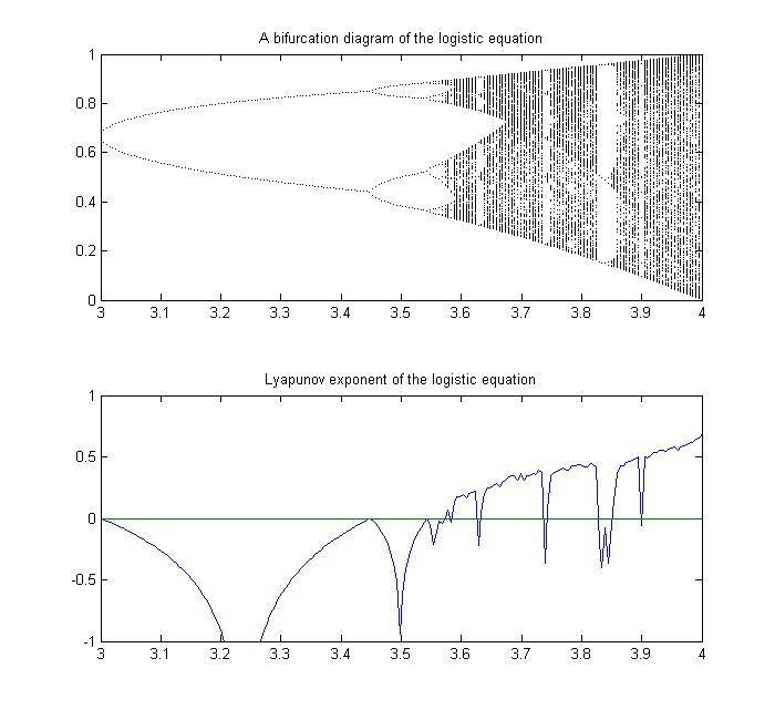
No comments:
Post a Comment